A data loader for the MVTec dataset
In this post, we introduce a data loader for the MVTec dataset, a dataset for benchmarking anomaly detection methods with a focus on industrial inspection.
The problem
Anomaly detection is one of the most fundamental problems in Machine Learning. Although it has different ‘flavors’, and there exists different techniques to approach it, the underlying problem is the same: to detect rare occurrences or observations which deviate from a common behavior and do not follow an established pattern. It has numerous applications in cyber-security, finance, computer vision and industrial inspection, among others.
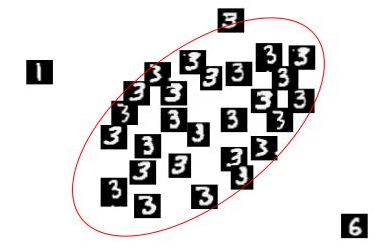
Figure 1. MNIST digit '3' with '1' and '6' anomalies
The MVTec dataset
Paraphrasing from the company’s website: ‘MVTec AD is a dataset for benchmarking anomaly detection methods with a focus on industrial inspection. It contains over 5000 high-resolution images divided into fifteen different object and texture categories. Each category comprises a set of defect-free training images and a test set of images with various kinds of defects as well as images without defects. Pixel-precise annotations of all anomalies are also provided’.
More precisely, the MVTec dataset is a dataset composed of 5354 high resolution square images of different objects, comprising 15 categories with 3629 images for training and validation, and 1725 images for testing. The training set only contains normal, i.e., defect-free images (label 1) and the test set contains both types of images: images containing various types of defects (label 0) and defect-free images. The anomalies manifest themselves in the form of over 70 different types of defects such as scratches, dents, contaminations, and various structural changes. Additionally, pixel-precise ground truth regions for all anomalies are provided in the dataset.
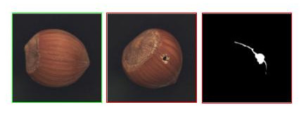
Figure 2. Normal, defective and ground truth samples for 'Hazelnut' category
The main reference for the dataset is the paper MVTec AD - A Comprehensive Real-World Dataset for Unsupervised Anomaly Detection, written by Bergmann and his collaborators. In this work, they introduce the dataset and also conduct a detailed evaluation of different unsupervised anomaly detection methods based on deep architectures such as convolutional autoencoders and generative adversarial networks, as well as classical computer vision methods. Table 1 in the paper gives a statistical overview for each category. Table 1 in this post is inspired from table 1 in the paper, with some additional relevant information, like the number of channels for each category.
Table 1. Statistical overview of the dataset
| Category | # Train | # Test (good) | # Test (defective) | Size | # Channels | |
|---|---|---|---|---|---|---|
| Textures | Carpet | 280 | 28 | 89 | 1024 | 3 |
| Grid | 264 | 21 | 57 | 1024 | 1 | |
| Leather | 245 | 32 | 92 | 1024 | 3 | |
| Tile | 230 | 33 | 84 | 840 | 3 | |
| Wood | 247 | 19 | 60 | 1024 | 3 | |
| Objects | Bottle | 209 | 20 | 63 | 900 | 3 |
| Cable | 224 | 58 | 92 | 1024 | 3 | |
| Capsule | 219 | 23 | 109 | 1000 | 3 | |
| Hazelnut | 391 | 40 | 70 | 1024 | 3 | |
| Metal nut | 220 | 22 | 93 | 700 | 3 | |
| Pill | 267 | 26 | 141 | 800 | 3 | |
| Screw | 320 | 41 | 119 | 1024 | 1 | |
| Toothbrush | 60 | 12 | 30 | 1024 | 3 | |
| Transistor | 213 | 60 | 40 | 1024 | 3 | |
| Zipper | 240 | 32 | 119 | 1024 | 1 | |
| Total | 3629 | 467 | 1258 | - | - |
The data loader
Popular datasets like MNIST or CIFAR10 have data loaders implemented in most frameworks like Pytorch and TensorFlow. However, due its novelty, an MVTec data loader has not yet been implemented in most frameworks. Because of this, my collaborator and I decided to implement a data loader for this dataset, inspired from TorchVision’s CIFAR10 data loader. The implementation can be found in this repo, as well as a jupyter notebook that works as a test and example of the data loader.
Main functionality
Using the data loader is as simple as import it
import mvtec
and start to use it
transform = transforms.Compose(
    [transforms.ToTensor()])

data = mvtec.MVTEC(root='./mvtec',
                   train=True,
                   transform=transform,
                   target_transform=None,
                   resize=64,
                   interpolation=3,
                   category='toothbrush')
The data loader has 7 input arguments. 3 of them are optional (transform, target_transform and resize), and all of them except ‘root’ have a default value. We can see a brief summary of the input arguments in table 2.
Table 2. Input arguments for data loader
| Argument | Optional? | Default value | Data type | Values |
|---|---|---|---|---|
| root | No | - | string | - |
| train | No | True | bool | [True, False] |
| transform | Yes | None | Callable | See next paragraph |
| target_transform | Yes | None | Callable | See next paragraph |
| resize | Yes | None | int | See next paragraph |
| interpolation | No | 2 | int | [0, 5] |
| category | No | ‘carpet’ | string | See next paragraph |
Specifically:
- ‘root’ is a string that specifies the root directory of dataset where directories ‘bottle’, ‘cable’, etc., exists.
- ‘train’ is a boolean that specifies which data to load, training or testing data
- ‘transform’ is a function/transform that takes in a PIL image and returns a transformed version of the image, for instance, ‘transforms.RandomCrop’. For more details see the test notebook
- ‘target_transform’ is a function/transform that takes in a label (1 or 0) and returns a transformed version of the label.
- ‘resize’ is an integer with the desired output image size (H=W=resize)
- ‘interpolation’ is an integer that specifies the interpolation method for downsizing the image. If ‘resize’ is not None, a value for interpolation must be provided. See this link for more details
- ‘category’ is a string specifying which data to load (bottle, cable, capsule, etc.)
Once the data loader has finished to load the data required, a message similar to the following message will be displayed:
original data shape: (N, H, W, C) (60, 1024, 1024, 3)
where N is the number of images loaded, H and W are the original image size (before resizing), and C is the number of channels in the images.
The data loader has two main functions: __len__ and __getitem__:
__len__simply returns the number of images loaded (i.e., N).__getitem__(index)returns a tuple: the index-th image and its corresponding label, after resizing and the corresponding transformations.
Figure 3 shows a screenshot from the test notebook, where the training data from the toothbrush category was loaded, transforming the images to pytorch tensors of size 256x256x3, with the bicubic interpolation method (interpolation method number 3).
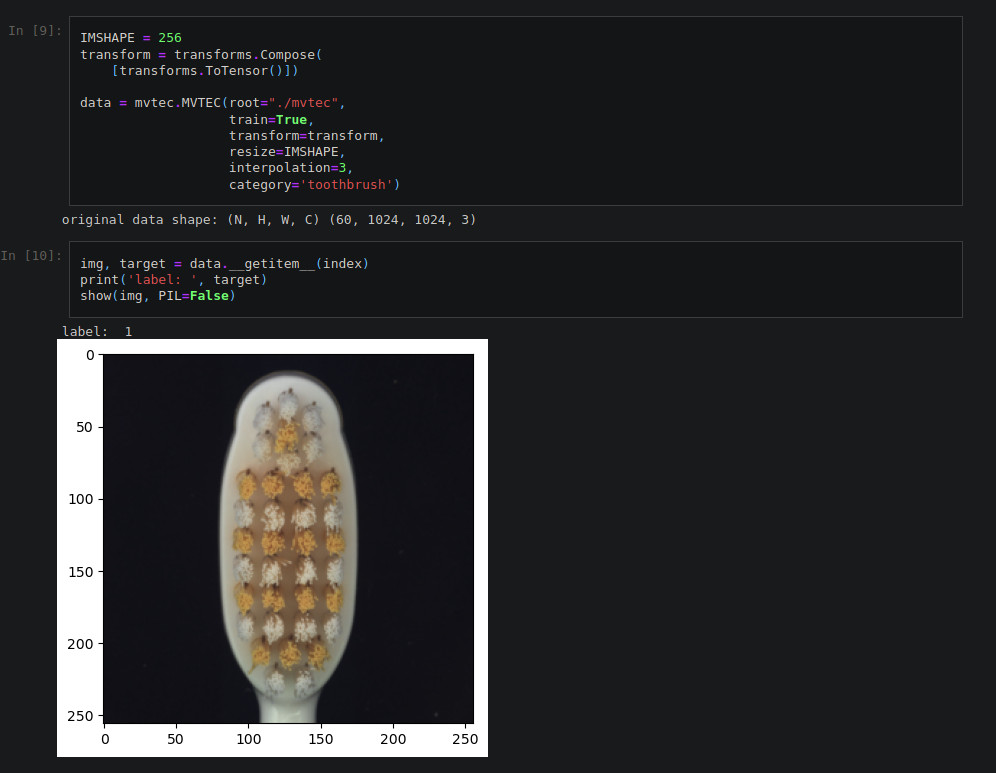
Figure 3. Loading toothbrush training images
Finally, the test notebook provides an example on how we can use the data loader in combination with the data loader from pytorch. Pytorch’s data loader takes the data loaded with our implementation and creates a new data loader with two main additional features (among others): it breaks the dataset in batches of a chosen size and it allows us to shuffle the data in the dataset. Figures 4 and 5 shows a couple of screenshots from the test notebook, where the test data from the pill category was loaded, transforming the images to pytorch tensors of size 128x128x3, with the bicubic interpolation method (interpolation method number 3). After that, a pytorch data loader is created with this data, breaking the dataset in batches of size 20.
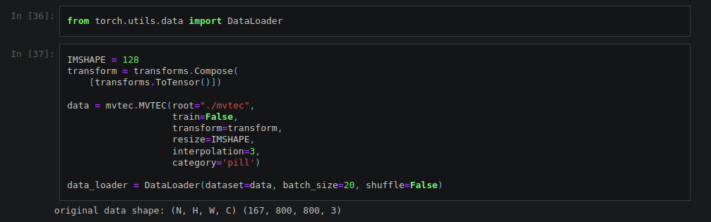
Figure 4. Loading pill test images
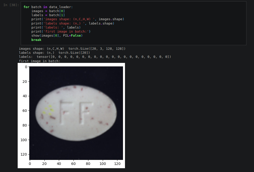
Figure 5. Using our data loader with pytorch's data loader
We hope that this implementation may be useful for the ML/AD/CV community, and we would like to hear your feedback.
Until our next post colegas,
B
References
- [1] Dataset
- [2] Short paper
- [3] Long paper
- [4] Papers with code link