Some brief notes about randomized algorithms
In this post, we share some notes about randomized algorithms and related ideas.
I spent some time the last few months looking for a Randomized Algorithms class to follow online. Luckily, I found the Randomized Algorithms class from UCSC, CSE290A Spring 2020, by Prof. Sesh Comandur. I’d the pleasure to meet him in person while I was studying at UCSC. I attended and enjoyed his Analysis of Boolean Functions class when I was in SC, so I decided to watch the lectures from his class.
This post will be an attempt to share a summary of what I consider the most important and interesting ideas from the lectures.

Figure 1. 'Randomized algorithm', image generated with DALL-E mini model
Some important concentration inequalities
- Markov’s inequality: given a non-negative random variable \( X \) and \( a > 0 \), then:
\[ P[X \geq a] \leq \frac{E[X]}{a} \]
- Chebyshev’s inequality: given a random variable \( X \) with finite non-zero variance \( \sigma^2 \) and \( a > 0 \), then:
\[ P[\lvert X - \mu \rvert \geq a\sigma] \leq \frac{1}{a^2} \]
- Hoeffding’s inequality: let \( X_1, …, X_n \) be independent random variables such that \( a_i \leq X_i \leq b_i \), and \( S = X_1+…+X_n \), then for all \( t > 0 \):
\[ P[S - E[S] \geq t] \leq \exp \left(-\frac{2t^2}{\sum (b_i-a_i)^2} \right) \] \[ P[\lvert S - E[S] \rvert \geq t] \leq 2\exp \left(-\frac{2t^2}{\sum (b_i-a_i)^2} \right) \]
- Generic Chernoff bounds: given a random variable \( X \) and \( t > 0 \), we can apply Markov’s inequality to the random variable \( e^{tX} \):
\[ P[X \geq a] = P[e^{tX} \geq e^{ta}] \leq E[ e^{tX} ]e^{-ta} \]
Since this bound holds for every positive \( t \), we may take the minimum:
\[ P[X \geq a] \leq \min_{t > 0} E[ e^{tX} ]e^{-ta} \]
Similarly, for the other tail:
\[ P[X \leq a] \leq \min_{t < 0} E[ e^{tX} ]e^{-ta} \]
The quantity \( E[ e^{tX} ] \) it’s called the moment-generating function, and it have some important properties, the most relevant being that it uniquely determines the distribution of \( X \).
- Multiplicative Chernoff bounds: let \( X_1, …, X_n \) be independent random variables taking values in {\( 0,1 \)}, let \( S = X_1+…+X_n \), and let \( \mu = E[S] \). Then for any \( \delta > 0 \):
\[ P[S \geq (1+\delta)\mu] < \left(\frac{e^{\delta}}{(1+\delta)^{1+\delta}} \right)^{\mu} \leq \exp \left(-\frac{\mu\delta^2}{3} \right) \]
Similarly, for the other tail (for any \( 1 > \delta > 0 \)):
\[ P[S \leq (1-\delta)\mu] < \left(\frac{e^{-\delta}}{(1-\delta)^{1-\delta}} \right)^{\mu} \leq \exp \left(-\frac{\mu\delta^2}{2} \right) \]
- Union bound: let \( E_1, …, E_n \) be a set of events with probabilities \( P[ E_1 ], …, P[ E_n ] \), respectively. Then:
\[ P \left[ \bigcup E_i \right] \leq \sum P[ E_i ] \]
Proofs for the majority of the inequalities mentioned can be found in wikipedia. A list of useful inequalities can be found in this cheatsheet.
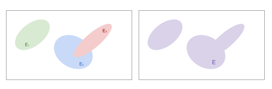
Figure 2. Union bound
Approximations to binomial \( B(n,p) \) distribution
-
Poisson limit theorem: if \( np \) converges to a finit limit \( \lambda \), then Poisson distribution \( Pois(\lambda) \) may be used as an approximation to the binomial distribution when \( n \to \infty \)
-
de Moivre–Laplace theorem: Normal distribution \( \mathcal{N}(np,\,np(1-p)) \) may be used as an approximation to the binomial distribution when \( n \to \infty \) (this is a special case of the CLT)
The Median trick
Used to boost the confidence of a randomized algorithm: given an algorithm that generates an output with confidence (i.e., probability of being correct) at least \( \frac{1}{2} \), run the algorithm \( O \left(\log \left(\frac{1}{\delta} \right) \right) \) times, and return the median output of such runs. The confidence of this procedure is at least \( 1-\delta \)
Walker’s alias method
Create a data structure to efficiently sample (\( O(1) \)) from a discrete probability distribution.
- \( O(n) \) preprocessing time
- Analogy with a liquid:
- \( n \) buckets with \( p_i \) liquid on them
- Immiscible liquids
- Transform it to n buckets with:
- \( \frac{1}{n} \) liquid on each of them
- At most 2 different liquids at each bucket
- \( q_1, q_2, …, q_n \)
- How? Walker’s alias method.
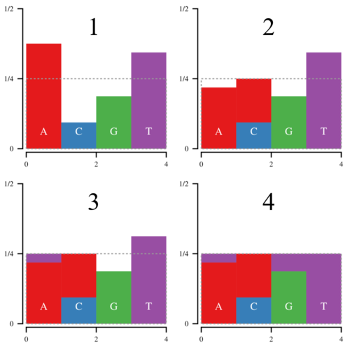
Figure 3. Walker’s alias method. Image taken from [7]
Erdos-Gallai theorem
Necessary and sufficient condition for a finite sequence of natural numbers to be the degree sequence of a graph

Figure 4. 'Men in suit with multiple hands', image generated with DALL-E mini model
Birthday paradox
Given a set with \( n \) items, choose \( m \) of them u.a.r (uniformly at random).
- If \( m \gg \sqrt{n} \), w.h.p. (with high probability) there is a collision (i.e., two persons share birthday)
- If \( m \ll \sqrt{n} \), w.h.p. there is no collision (i.e., no shared birthday)
- For instance, given a common year, we have \( n = 365 \) days. The square root of n is \( \sqrt{365} \approx 19 \). In a reunion with \( 10 \) people, the probability of two persons sharing birthday is approximately 0.117. On the other hand, in a reunion with \( 40 \) people, the probability of two persons sharing birthday is approximately 0.891.
- Brain teaser: you have a million of empty buckets in front of you, and you throw (let’s say) three thousand of balls at them. Three thousand is not even one percent of one million. Assuming that the probability for each ball of landing at any bucket is the same, what is the probability of a collision (i.e., at least one bucket having more than one ball)?
Coupon collector
Given a set with \( n \) items, how many items do you expect you need to draw with replacement before having drawn each coupon at least once?
- The expected number of trials needed grows as \( \Theta(n\log(n)) \)
- More precisely: \( E[ T ] = n\log(n) + \gamma n + \frac{1}{2} + O(\frac{1}{n}) \), where \( \gamma \approx 0.5772 \) is the Euler–Mascheroni constant.
Reservoir sampling
A simple and elegant idea on how to sample u.a.r. from a streaming of \( n \) items, where we don’t know in advance the value of \( n \).
- To sample one element u.a.r. from a stream S, simply store one element
- On seeing the \( t-th \) element of the stream (i.e., \( S[t] \), 1-based indexing) replace stored element by \( S[t] \) with probability \( \frac{1}{t} \).
Some other important ideas that deserve their own post
Some of the lectures covered very important techniques and ideas that deserve their own post. I don’t promise anything, but hopefully we will see a post about them in the future. A glimpse of these ideas: estimating the average degree of a graph, the JL Lemma, Poissonization, Uniformity testing, the HHL algorithm, among others.
Some implementations
I implemented some of the algorithms studied in the lectures. I’m still delighted by the Karp-Luby-Madras algorithm. You can find the python implementations here.
Until our next post colegas,
B
References
- [1] Lectures playlist
- [2] DALL-E mini model
- [3] Concentration inequalities
- [4] Poisson limit theorem
- [5] de Moivre–Laplace theorem
- [6] Median trick
- [7] Panda’s Thumb
- [8] Erdos-Gallai theorem
- [9] Birthday paradox
- [10] Coupon collector
- [11] Reservoir sampling